MATLAB, 1st order 2d hyperbolic equation, problem with convergence.

Question

Follow up to my previous question: MATLAB: solving 1st order hyperbolic equation in 2 spacial dimensions

The equation I'm solving has the form: $$f_t + A y f_x - B x f_y =0$$

I wrote the following code according to the comments from the previous question:

% Liouville equation
clear;

% Equation Parameters:
Xmin = -10.0; % Minimum X
Ymin = -10.0; % Minimum Y
Xmax = 10.0; % Maximum X
Ymax = 10.0; % Maximum Y
Tmax = 1.0; % Maximum time
A = 1.0;    % A parameter
B = 1.0;    % B parameter

% Simulation parameters:
Nt = 1000; % Number of time steps
dt = Tmax/Nt;

Nx = 200; % Number of X space steps
dx = (Xmax-Xmin)/Nx;

Ny = 200; % Number of X space steps
dy = (Ymax-Ymin)/Ny;

dtdx = dt/dx;   % For simplicity
dtdy = dt/dy;

% Filling the x,y steps
for i=1:(Nx+1)
x(i) = Xmin + (i-1)*dx;
end

for j=1:(Ny+1)
y(j) = Ymin + (j-1)*dy;
end

% Initial condition
for i = 1:(Nx+1)
    for j = 1:(Ny+1)
        u(i,j,1)=uzero(x(i),y(j),1.0,0.0,0.25,0.25);
    end
end

% Boundary condition
for k=1:(Nt+1)
    u(1,1,k) = 0;
    u(Nx+1,Ny+1,k) = 0;
    t(k) = (k-1)*dt;
end

% Time stepping algorithm
for k=1:Nt                                      % Time loop
    for i=2:Nx                                  % Space loop
        for j=2:Ny                              % Space loop
            u(i,j,k+1) = u(i,j,k)- 0.5*A*dtdx*y(j)*(u(i+1,j,k)-u(i-1,j,k)) - 0.5*B*dtdy*x(i)*(u(i,j+1,k)-u(i,j-1,k));
        end
    end
end

% Graphical representation of the function
[x,y] = meshgrid(x,y);


for m=1:9
   subplot(3,3,m);
   surf(x,y,u(:,:,round(m*Nt/9)));
   zlim([0 1]);
   shading interp;
end

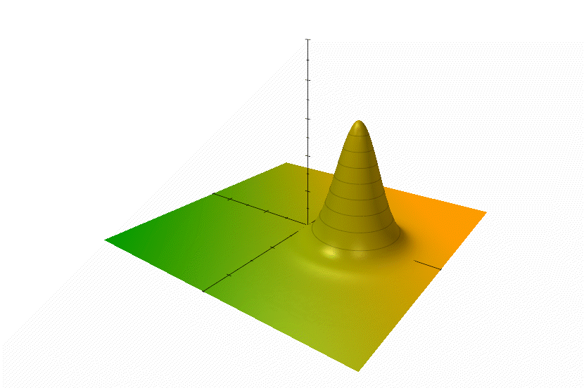
The uzero function is a gaussian. I'm using one centered at $(1,0)$ with standard deviations $0.25$. This is the result of the plots at 9 different points in time:

The theoretical behaviour of this should be this: (http://upload.wikimedia.org/wikipedia/commons/d/d6/DisplacedGaussianWF.gif). Clearly this isn't the case, the Gaussian loses its shape (becomes flat). I've checked the scheme and I don't see any mistakes in implementation. So my questions are:

1. What's wrong? Is it some mistake in the code I didn't catch or is the used solution scheme too primitive? Even small changes in the paramaters sometimes produce completely bizzare results, so it looks to me like a stability problem.

2. Is there a better way of implementing this algorithm? It runs very slowly for me, even with relatively small amounts of steps.

Answer 1

There was one important mistake in the code, you had +B as the coefficient for the $f_y$ part, not -B. Other than that, I've gone through and removed a lot of for loops by doing vector operations. This speeds the code up quite a bit. I don't have the uzero function so I used mvnpdf.

The stability is quite poor, reducing the time step helps, but a higher-order method for approximating the derivatives might be required if reducing the time step isn't enough, or if the accuracy isn't good enough.

The only for loop required is for the time stepping, since we use results from the previous step to determine the current values, but for the spatial stepping we are using already known values, so it can be done in one go.

Here's my modified code. This should be more accurate and run faster than your code, but it does the same steps:

%// Liouville equation
clear;

%// Equation Parameters:
Xmin = -10.0; %// Minimum X
Ymin = -10.0; %// Minimum Y
Xmax = 10.0;  %// Maximum X
Ymax = 10.0;  %// Maximum Y
Tmin=0;       %// Minimum time
Tmax = 5.0;   %// Maximum time
A = 1.0;      %// A parameter
B = 1.0;      %// B parameter

%// Simulation parameters:
Nt = 2000; %// Number of time steps
Nx = 100;  %// Number of X space steps
Ny = 100;  %// Number of X space steps

%// Create time and space vectors with exactly Nt, Nx, Ny elements
t=linspace(Tmin,Tmax,Nt);
x=linspace(Xmin,Xmax,Nx);
y=linspace(Ymin,Ymax,Ny);

%// Make a grid of x and y coordinates    
[X,Y] = ndgrid(x,y);

%// Calculate dt, dx and dy
dt=t(2)-t(1);
dx=x(2)-x(1);
dy=y(2)-y(1);

dtdx = dt/dx;   %// For simplicity
dtdy = dt/dy;

u=zeros(Nx,Ny,Nt); %// Initialise u matrix

%// Initial condition
u(:,:,1)=reshape(mvnpdf([X(:),Y(:)],[1.0 ,0.0],[0.25,0.25]),Nx,Ny);

%// Time stepping algorithm
i=2:Nx-1; %// Interior spatial points
j=2:Ny-1;
for k=2:Nt
    u(i,j,k) = u(i,j,k-1) - 0.5*A*dtdx*Y(i,j).*(u(i+1,j,k-1)-u(i-1,j,k-1)) ...
        + 0.5*B*dtdy*X(i,j).*(u(i,j+1,k-1)-u(i,j-1,k-1));
end

%// Animate the solution
for m=1:10:Nt
   surf(x,y,u(:,:,m))
   title(num2str(t(m)))
   shading interp;
   drawnow()
   pause(0.1)
end